Building blueprints programmatically

For maximum control and automation, you can define Blueprints in code using the Python Blueprint API. This is ideal for:

Creating layouts dynamically based on your data
Ensuring consistent views for specific debugging scenarios
Generating complex layouts that would be tedious to build manually
Sending different blueprints based on runtime conditions

Getting started example getting-started-example

This walkthrough demonstrates the Blueprint API using stock market data. We'll start simple and progressively build more complex layouts.

Setup

First, create a virtual environment and install dependencies:

Linux/Mac:

python -m venv venv
source venv/bin/activate
pip install rerun-sdk humanize yfinance

Windows:

python -m venv venv
.\venv\Scripts\activate
pip install rerun-sdk humanize yfinance

Basic script

Create stocks.py with the necessary imports:

#!/usr/bin/env python3
import datetime as dt
import humanize
import pytz
import yfinance as yf
from typing import Any

import rerun as rr
import rerun.blueprint as rrb

Add helper functions for styling:

brand_colors = {
    "AAPL": 0xA2AAADFF,
    "AMZN": 0xFF9900FF,
    "GOOGL": 0x34A853FF,
    "META": 0x0081FBFF,
    "MSFT": 0xF14F21FF,
}

def style_plot(symbol: str) -> rr.SeriesLine:
    return rr.SeriesLine(
        color=brand_colors[symbol],
        name=symbol,
    )

def style_peak(symbol: str) -> rr.SeriesPoint:
    return rr.SeriesPoint(
        color=0xFF0000FF,
        name=f"{symbol} (peak)",
        marker="Up",
    )

def info_card(
    shortName: str,
    industry: str,
    marketCap: int,
    totalRevenue: int,
    **args: dict[str, Any],
) -> rr.TextDocument:
    markdown = f"""
- **Name**: {shortName}
- **Industry**: {industry}
- **Market cap**: ${humanize.intword(marketCap)}
- **Total Revenue**: ${humanize.intword(totalRevenue)}
"""
    return rr.TextDocument(markdown, media_type=rr.MediaType.MARKDOWN)

Add the main function that logs data:

def main() -> None:
    symbols = ["AAPL", "AMZN", "GOOGL", "META", "MSFT"]

    # Use eastern time for market hours
    et_timezone = pytz.timezone("America/New_York")
    start_date = dt.date(2024, 3, 18)
    dates = [start_date + dt.timedelta(days=i) for i in range(5)]

    # Initialize Rerun and spawn a new viewer
    rr.init("rerun_example_blueprint_stocks", spawn=True)

    # This is where we will edit the blueprint
    blueprint = None
    #rr.send_blueprint(blueprint)

    # Log the stock data for each symbol and date
    for symbol in symbols:
        stock = yf.Ticker(symbol)

        # Log the stock info document as static
        rr.log(f"stocks/{symbol}/info", info_card(**stock.info), static=True)

        for day in dates:
            # Log the styling data as static
            rr.log(f"stocks/{symbol}/{day}", style_plot(symbol), static=True)
            rr.log(f"stocks/{symbol}/peaks/{day}", style_peak(symbol), static=True)

            # Query the stock data during market hours
            open_time = dt.datetime.combine(day, dt.time(9, 30), et_timezone)
            close_time = dt.datetime.combine(day, dt.time(16, 00), et_timezone)

            hist = stock.history(start=open_time, end=close_time, interval="5m")

            # Offset the index to be in seconds since the market open
            hist.index = hist.index - open_time
            peak = hist.High.idxmax()

            # Log the stock state over the course of the day
            for row in hist.itertuples():
                rr.set_time("time", duration=row.Index)
                rr.log(f"stocks/{symbol}/{day}", rr.Scalars(row.High))
                if row.Index == peak:
                    rr.log(f"stocks/{symbol}/peaks/{day}", rr.Scalars(row.High))

if __name__ == "__main__":
    main()

Run the script:

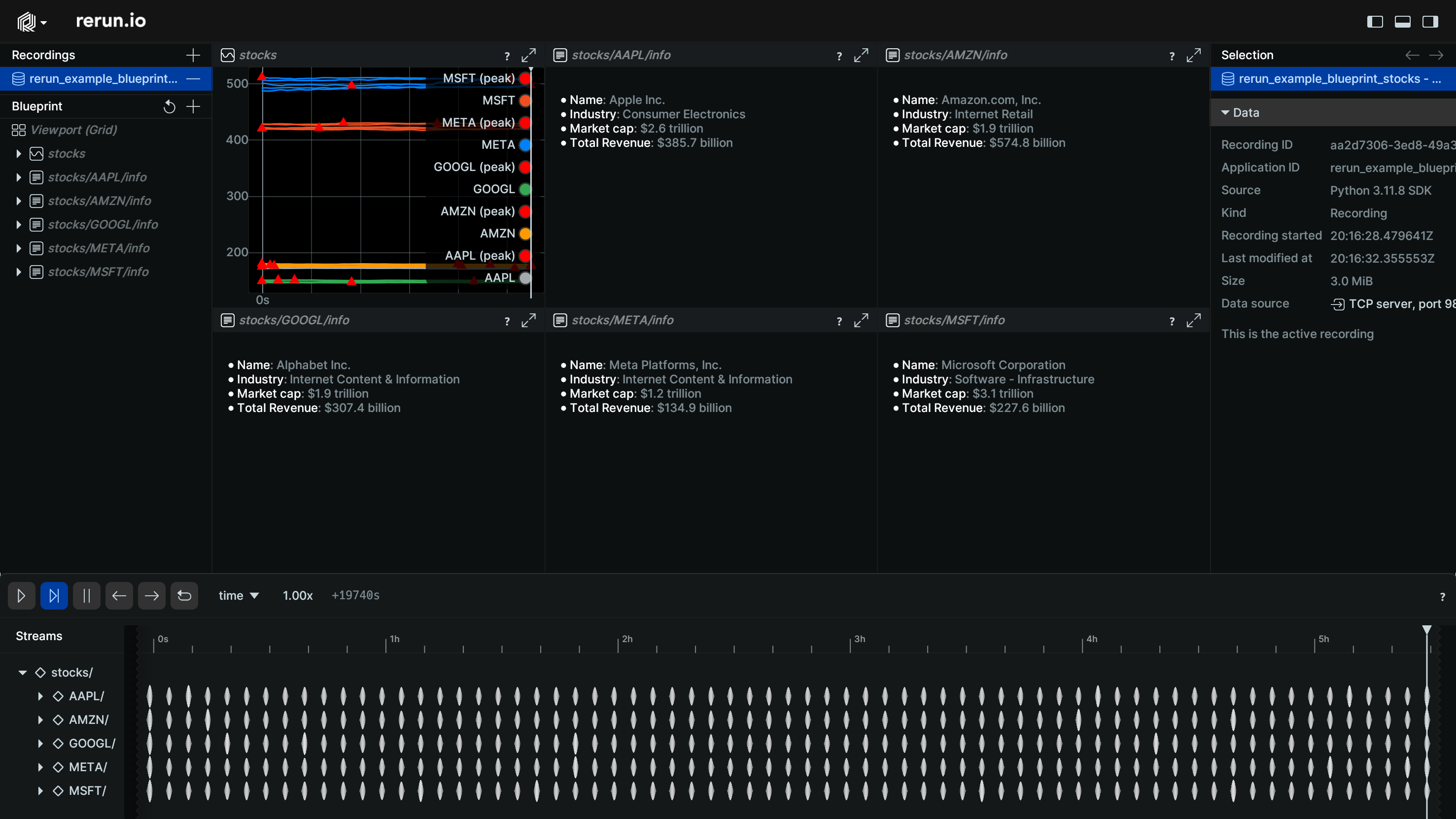
python stocks.py

Without a blueprint, the heuristic layout may not be ideal:

Creating a simple view creating-a-simple-view

Replace the blueprint section with:

# Create a single chart for all the AAPL data:
blueprint = rrb.Blueprint(
    rrb.TimeSeriesView(name="AAPL", origin="/stocks/AAPL"),
)
rr.send_blueprint(blueprint)

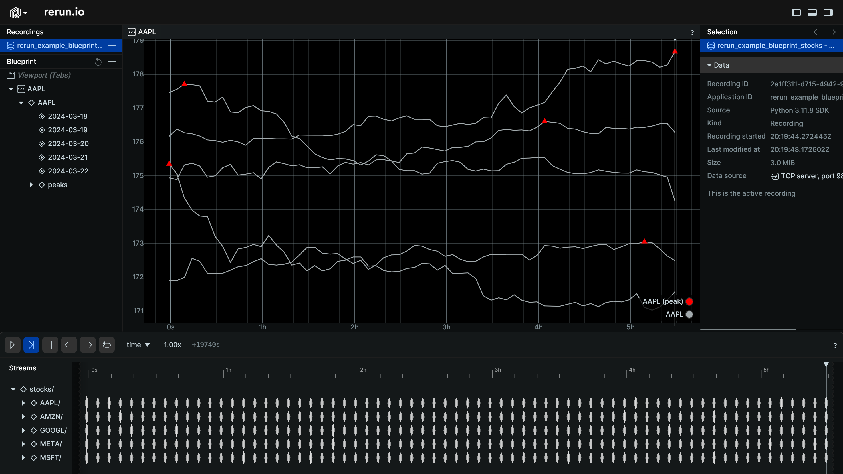
The origin parameter scopes the view to a specific subtree. Now you'll see just the AAPL data:

Controlling panel state controlling-panel-state

You can control which panels are visible:

# Create a single chart and collapse the selection and time panels:
blueprint = rrb.Blueprint(
    rrb.TimeSeriesView(name="AAPL", origin="/stocks/AAPL"),
    rrb.BlueprintPanel(state="expanded"),
    rrb.SelectionPanel(state="collapsed"),
    rrb.TimePanel(state="collapsed"),
)
rr.send_blueprint(blueprint)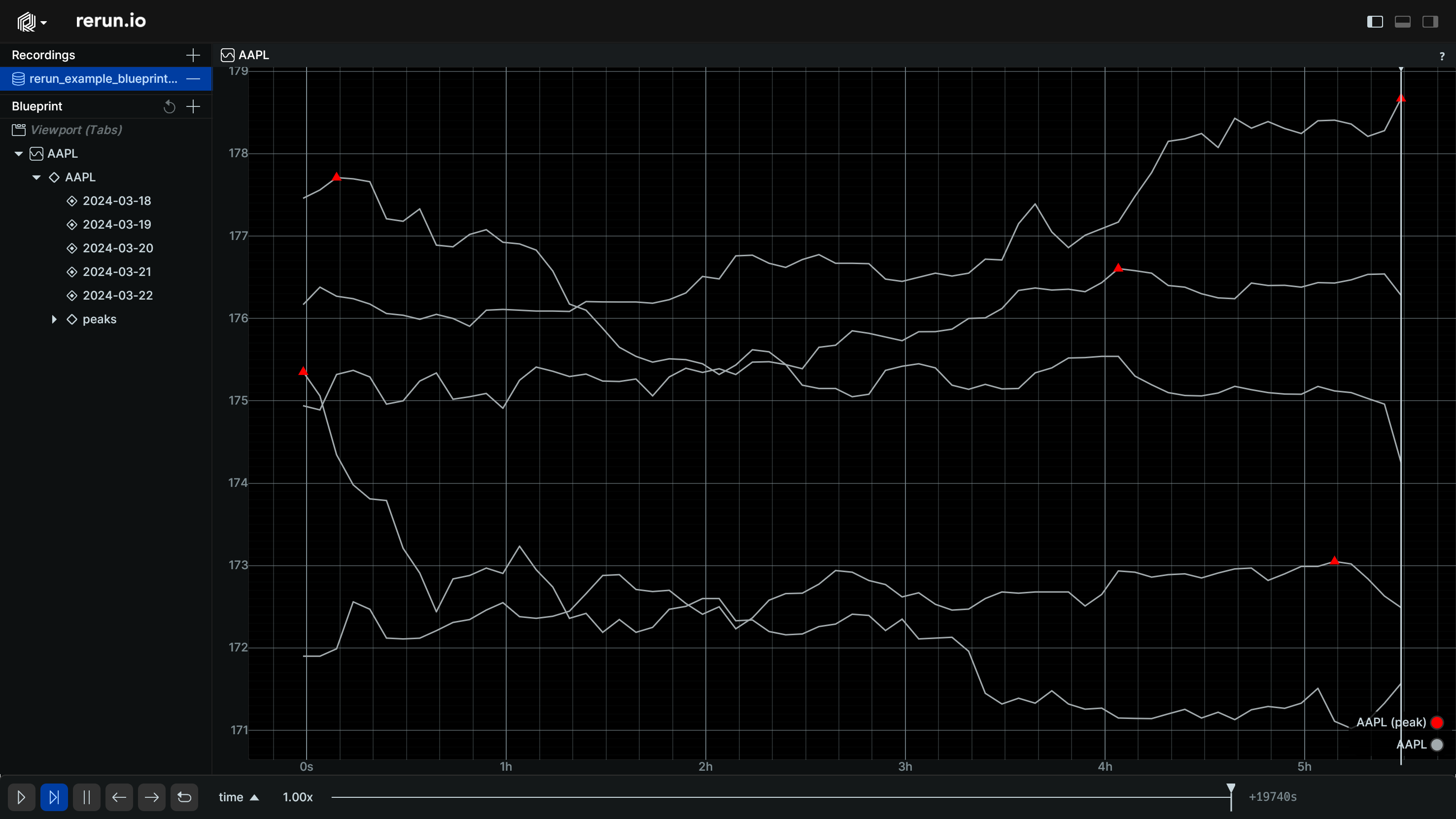

Combining multiple views combining-multiple-views

Use containers to combine multiple views. The Vertical container stacks views, and row_shares controls relative sizing:

# Create a vertical layout of an info document and a time series chart
blueprint = rrb.Blueprint(
    rrb.Vertical(
        rrb.TextDocumentView(name="Info", origin="/stocks/AAPL/info"),
        rrb.TimeSeriesView(name="Chart", origin="/stocks/AAPL"),
        row_shares=[1, 4],
    ),
    rrb.BlueprintPanel(state="expanded"),
    rrb.SelectionPanel(state="collapsed"),
    rrb.TimePanel(state="collapsed"),
)
rr.send_blueprint(blueprint)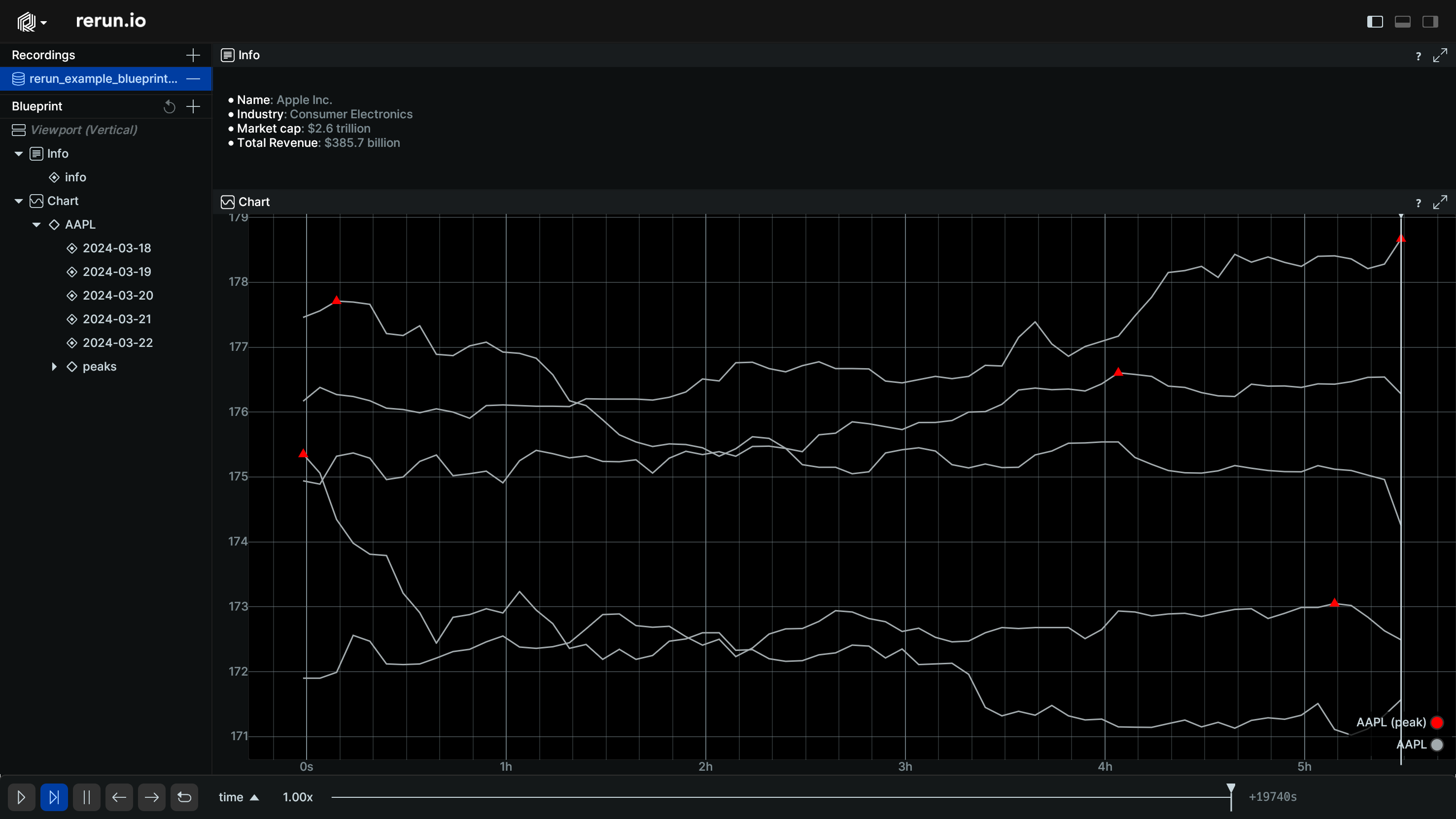

Specifying view contents specifying-view-contents

The contents parameter provides fine-grained control over what appears in a view. You can include data from multiple sources:

# Create a view with two stock time series
blueprint = rrb.Blueprint(
    rrb.TimeSeriesView(
        name="META vs MSFT",
        contents=[
            "+ /stocks/META/2024-03-19",
            "+ /stocks/MSFT/2024-03-19",
        ],
    ),
    rrb.BlueprintPanel(state="expanded"),
    rrb.SelectionPanel(state="collapsed"),
    rrb.TimePanel(state="collapsed"),
)
rr.send_blueprint(blueprint)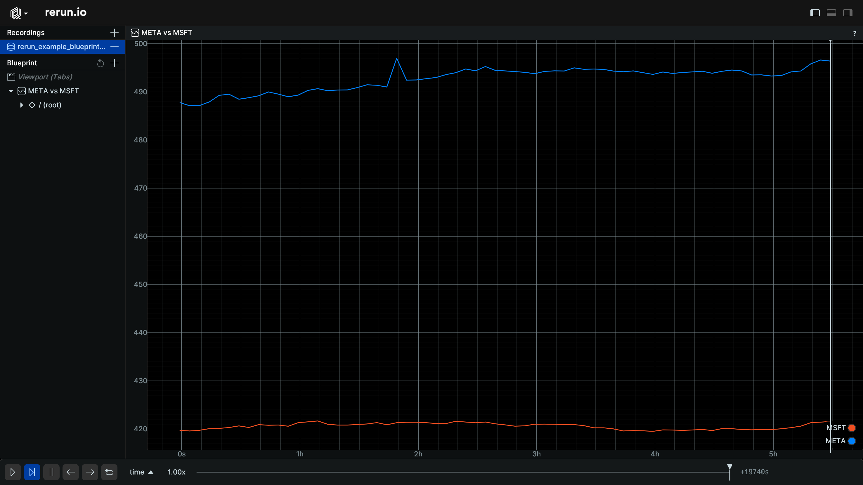

Filtering with expressions filtering-with-expressions

Content expressions can include or exclude subtrees using wildcards. They can reference $origin and use /** to match entire subtrees:

# Create a chart for AAPL and filter out the peaks:
blueprint = rrb.Blueprint(
    rrb.TimeSeriesView(
        name="AAPL",
        origin="/stocks/AAPL",
        contents=[
            "+ $origin/**",
            "- $origin/peaks/**",
        ],
    ),
    rrb.BlueprintPanel(state="expanded"),
    rrb.SelectionPanel(state="collapsed"),
    rrb.TimePanel(state="collapsed"),
)
rr.send_blueprint(blueprint)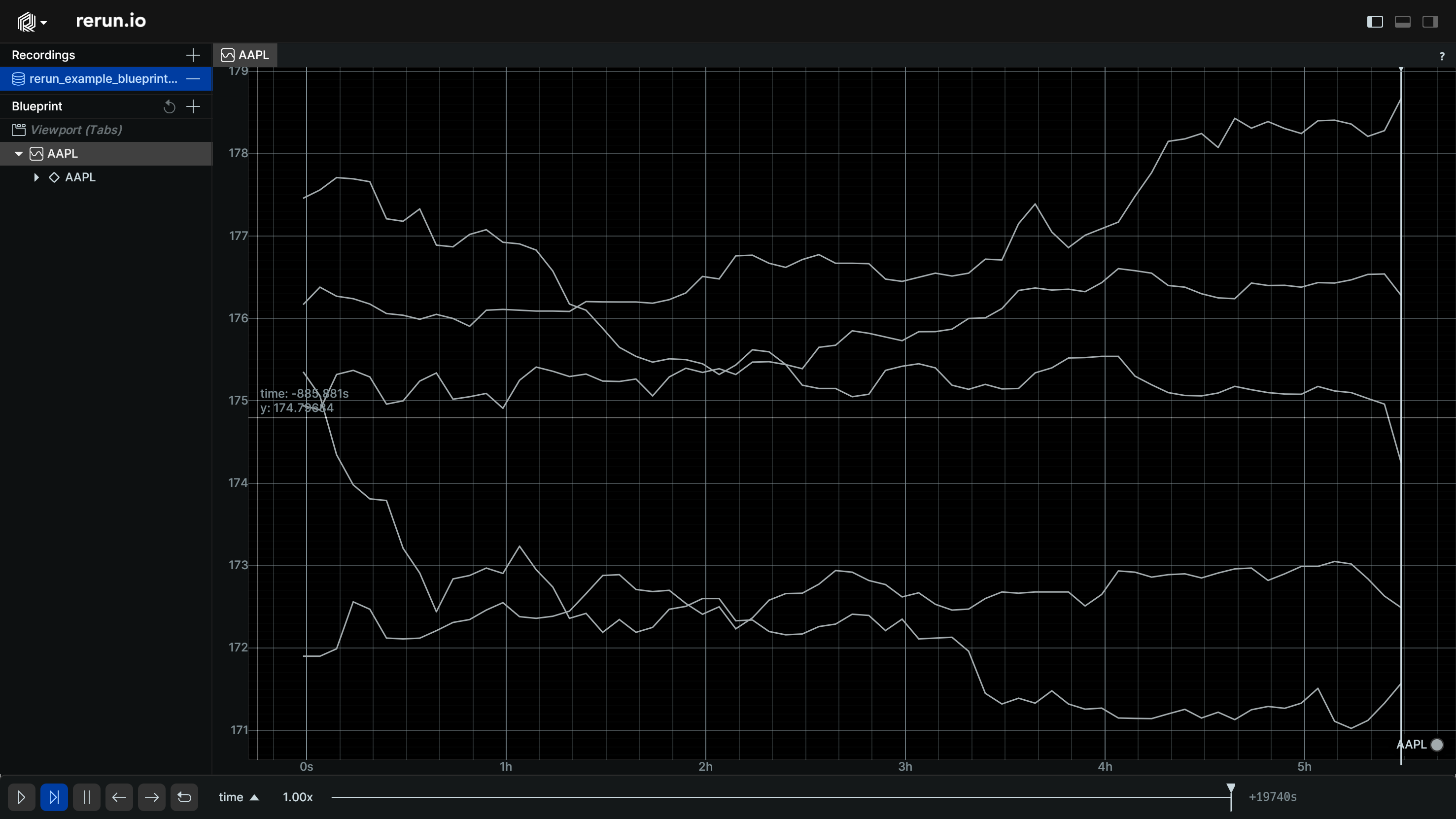

See Entity Queries for complete expression syntax.

Programmatic layout generation programmatic-layout-generation

Since blueprints are Python code, you can generate them dynamically. This example creates a grid with one row per stock symbol:

# Iterate over all symbols and days to create a comprehensive grid
blueprint = rrb.Blueprint(
    rrb.Vertical(
        contents=[
            rrb.Horizontal(
                contents=[
                    rrb.TextDocumentView(
                        name=f"{symbol}",
                        origin=f"/stocks/{symbol}/info",
                    ),
                ]
                + [
                    rrb.TimeSeriesView(
                        name=f"{day}",
                        origin=f"/stocks/{symbol}/{day}",
                    )
                    for day in dates
                ],
                name=symbol,
            )
            for symbol in symbols
        ]
    ),
    rrb.BlueprintPanel(state="expanded"),
    rrb.SelectionPanel(state="collapsed"),
    rrb.TimePanel(state="collapsed"),
)
rr.send_blueprint(blueprint)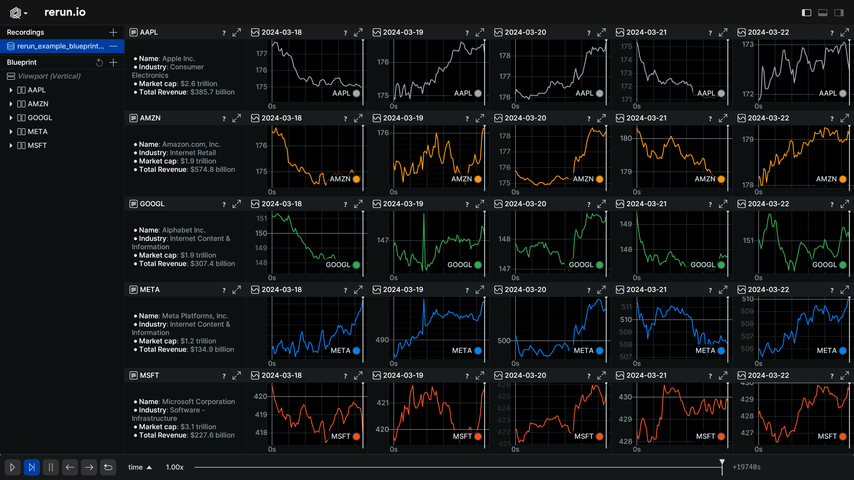

Saving blueprints from code saving-blueprints-from-code

You can save programmatically-created blueprints to .rbl files:

blueprint = rrb.Blueprint(
    rrb.TimeSeriesView(name="AAPL", origin="/stocks/AAPL"),
)

# Save to a file
blueprint.save("rerun_example_blueprint_stocks", "my_blueprint.rbl")

# Later, load it in any language
rr.log_file_from_path("my_blueprint.rbl")

Loading blueprints from any language

The programmatic way works by calling log_file_from_path:

This method allows you to log any file that contains data that Rerun understands (in this case, blueprint data) as part of your current recording.

This enables reusing blueprints across different programming languages. See the Blueprint API Reference for complete details.

Advanced customization advanced-customization

Blueprints support deep customization of view properties. For example:

# Configure a 3D view with custom camera settings
rrb.Spatial3DView(
    name="Robot view",
    origin="/world/robot",
    background=[100, 149, 237],  # Light blue
    eye_controls=rrb.EyeControls3D(
        kind=rrb.Eye3DKind.FirstPerson,
        speed=20.0,
    ),
)

# Configure a time series view with custom axis and time ranges
rrb.TimeSeriesView(
    name="Sensor Data",
    origin="/sensors",
    axis_y=rrb.ScalarAxis(range=(-10.0, 10.0), zoom_lock=True),
    plot_legend=rrb.PlotLegend(visible=False),
    time_ranges=[
        rrb.VisibleTimeRange(
            "time",
            start=rrb.TimeRangeBoundary.cursor_relative(seq=-100),
            end=rrb.TimeRangeBoundary.cursor_relative(),
        ),
    ],
)

See Visualizers and Overrides for information on overriding component values and controlling visualizers from code.

Youtube overview youtube-overview

While some people might want to read through the documentation on this page, others might prefer to watch a video! If you would like to follow along with the Youtube video, you can find the code used in the video below.

from __future__ import annotations

import math

import numpy as np
import rerun as rr
import rerun.blueprint as rrb
from numpy.random import default_rng

rr.init("rerun_blueprint_example", spawn=True)

rr.set_time("time", sequence=0)
rr.log("log/status", rr.TextLog("Application started.", level=rr.TextLogLevel.INFO))
rr.set_time("time", sequence=5)
rr.log("log/other", rr.TextLog("A warning.", level=rr.TextLogLevel.WARN))
for i in range(10):
    rr.set_time("time", sequence=i)
    rr.log(
        "log/status", rr.TextLog(f"Processing item {i}.", level=rr.TextLogLevel.INFO)
    )

# Create a text view that displays all logs.
blueprint = rrb.Blueprint(
    rrb.TextLogView(origin="/log", name="Text Logs"),
    rrb.SelectionPanel(state="expanded"),
    collapse_panels=True,
)

rr.send_blueprint(blueprint)


input("Press Enter to continue…")

# Create a spiral of points:
n = 150
angle = np.linspace(0, 10 * np.pi, n)
spiral_radius = np.linspace(0.0, 3.0, n) ** 2
positions = np.column_stack(
    (np.cos(angle) * spiral_radius, np.sin(angle) * spiral_radius)
)
colors = np.dstack(
    (np.linspace(255, 255, n), np.linspace(255, 0, n), np.linspace(0, 255, n))
)[0].astype(int)
radii = np.linspace(0.01, 0.7, n)

rr.log("points", rr.Points2D(positions, colors=colors, radii=radii))

# Create a Spatial2D view to display the points.
blueprint = rrb.Blueprint(
    rrb.Spatial2DView(
        origin="/",
        name="2D Scene",
        # Set the background color
        background=[105, 20, 105],
        # Note that this range is smaller than the range of the points,
        # so some points will not be visible.
        visual_bounds=rrb.VisualBounds2D(x_range=[-5, 5], y_range=[-5, 5]),
    ),
    collapse_panels=True,
)

rr.send_blueprint(blueprint)


input("Press Enter to continue…")

rr.log(
    "points",
    rr.GeoPoints(
        lat_lon=[[47.6344, 19.1397], [47.6334, 19.1399]],
        radii=rr.Radius.ui_points(20.0),
    ),
)

# Create a map view to display the chart.
blueprint = rrb.Blueprint(
    rrb.MapView(
        origin="points",
        name="MapView",
        zoom=16.0,
        background=rrb.MapProvider.OpenStreetMap,
    ),
    collapse_panels=True,
)


rr.send_blueprint(blueprint)

input("Press Enter to continue…")

blueprint = rrb.Blueprint(
    rrb.Grid(
        rrb.MapView(
            origin="points",
            name="MapView",
            zoom=16.0,
            background=rrb.MapProvider.OpenStreetMap,
        ),
        rrb.Spatial2DView(
            origin="/",
            name="2D Scene",
            # Set the background color
            background=[105, 20, 105],
            # Note that this range is smaller than the range of the points,
            # so some points will not be visible.
            visual_bounds=rrb.VisualBounds2D(x_range=[-5, 5], y_range=[-5, 5]),
        ),
        rrb.TextLogView(origin="/log", name="Text Logs"),
    ),
    rrb.TimePanel(state="expanded"),
    rrb.BlueprintPanel(state="expanded"),
    collapse_panels=True,
)

rr.send_blueprint(blueprint)

blueprint.save("my_favorite_blueprint", "data/blueprint.rbl")

input("Press Enter to continue…")


rr.log("bar_chart", rr.BarChart([8, 4, 0, 9, 1, 4, 1, 6, 9, 0]))

rng = default_rng(12345)
positions = rng.uniform(-5, 5, size=[50, 3])
colors = rng.uniform(0, 255, size=[50, 3])
radii = rng.uniform(0.1, 0.5, size=[50])

rr.log("3dpoints", rr.Points3D(positions, colors=colors, radii=radii))

tensor = np.random.randint(0, 256, (32, 240, 320, 3), dtype=np.uint8)
rr.log("tensor", rr.Tensor(tensor, dim_names=("batch", "x", "y", "channel")))

rr.log(
    "markdown",
    rr.TextDocument(
        """
# Hello Markdown!
[Click here to see the raw text](recording://markdown:Text).
"""
    ),
)

rr.log("trig/sin", rr.SeriesLines(colors=[255, 0, 0], names="sin(0.01t)"), static=True)
for t in range(int(math.pi * 4 * 100.0)):
    rr.set_time("time", sequence=t)
    rr.set_time("timeline1", duration=t)
    rr.log("trig/sin", rr.Scalars(math.sin(float(t) / 100.0)))

blueprint = rrb.Blueprint(
    rrb.Grid(
        rrb.MapView(
            origin="points",
            name="MapView",
            zoom=16.0,
            background=rrb.MapProvider.OpenStreetMap,
        ),
        rrb.Spatial2DView(
            origin="/",
            name="2D Scene",
            # Set the background color
            background=[105, 20, 105],
            # Note that this range is smaller than the range of the points,
            # so some points will not be visible.
            visual_bounds=rrb.VisualBounds2D(x_range=[-5, 5], y_range=[-5, 5]),
        ),
        rrb.TextLogView(origin="/log", name="Text Logs"),
        rrb.BarChartView(origin="bar_chart", name="Bar Chart"),
        rrb.Spatial3DView(
            origin="/3dpoints",
            name="3D Scene",
            # Set the background color to light blue.
            background=[100, 149, 237],
            # Configure the eye controls.
            eye_controls=rrb.EyeControls3D(
                kind=rrb.Eye3DKind.FirstPerson,
                speed=20.0,
            ),
        ),
        rrb.TensorView(
            origin="tensor",
            name="Tensor",
            # Explicitly pick which dimensions to show.
            slice_selection=rrb.TensorSliceSelection(
                # Use the first dimension as width.
                width=1,
                # Use the second dimension as height and invert it.
                height=rr.TensorDimensionSelection(dimension=2, invert=True),
                # Set which indices to show for the other dimensions.
                indices=[
                    rr.TensorDimensionIndexSelection(dimension=2, index=4),
                    rr.TensorDimensionIndexSelection(dimension=3, index=5),
                ],
                # Show a slider for dimension 2 only. If not specified, all dimensions in `indices` will have sliders.
                slider=[2],
            ),
            # Set a scalar mapping with a custom colormap, gamma and magnification filter.
            scalar_mapping=rrb.TensorScalarMapping(
                colormap="turbo", gamma=1.5, mag_filter="linear"
            ),
            # Fill the view, ignoring aspect ratio.
            view_fit="fill",
        ),
        rrb.TextDocumentView(origin="markdown", name="Markdown example"),
        rrb.TimeSeriesView(
            origin="/trig",
            # Set a custom Y axis.
            axis_y=rrb.ScalarAxis(range=(-1.0, 1.0), zoom_lock=True),
            # Configure the legend.
            plot_legend=rrb.PlotLegend(visible=False),
            # Set time different time ranges for different timelines.
            time_ranges=[
                # Sliding window depending on the time cursor for the first timeline.
                rrb.VisibleTimeRange(
                    "time",
                    start=rrb.TimeRangeBoundary.cursor_relative(seq=-100),
                    end=rrb.TimeRangeBoundary.cursor_relative(),
                ),
                # Time range from some point to the end of the timeline for the second timeline.
                rrb.VisibleTimeRange(
                    "timeline1",
                    start=rrb.TimeRangeBoundary.absolute(seconds=300.0),
                    end=rrb.TimeRangeBoundary.infinite(),
                ),
            ],
        ),
    ),
    collapse_panels=True,
)

rr.send_blueprint(blueprint)